Let ![]() be the the population of a given species at time
be the the population of a given species at time ![]() . The variation of population is the rate of change of
. The variation of population is the rate of change of ![]() is proportional to the current value of
is proportional to the current value of ![]() that is
that is

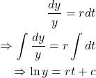
Where ![]() is the proportionality constant, called the rate of growth and decline depending on whether it is positive or negative. Let
is the proportionality constant, called the rate of growth and decline depending on whether it is positive or negative. Let ![]() , so the population is growing. This idea was published by the British economist Thomas Malthus (1766-1834) in 1798. From the above equation we get,
, so the population is growing. This idea was published by the British economist Thomas Malthus (1766-1834) in 1798. From the above equation we get,

where ![]() is an integrating constant.
is an integrating constant.

If ![]() then
then ![]() which implies
which implies
![]()
Malthus model with ![]() predicts that the population will grow exponentially for all time. Equation
predicts that the population will grow exponentially for all time. Equation ![]() is accurate for many populations at least for limited periods of time. However such ideal conditions can not continue indefinitely. Eventually limitations on space, food supply or other resources will reduce the growth rate and bring an end to uninhibited exponential growth.
is accurate for many populations at least for limited periods of time. However such ideal conditions can not continue indefinitely. Eventually limitations on space, food supply or other resources will reduce the growth rate and bring an end to uninhibited exponential growth.
Considering the fact that the growth rate actually depends on the population. We replace the constant ![]() by a function
by a function ![]() and thus we obtain the modified equation
and thus we obtain the modified equation
(L) ![]()
We now choose ![]() so that
so that ![]() when
when ![]() is small,
is small, ![]() decreases as
decreases as ![]() grows larger and
grows larger and ![]() when
when ![]() is sufficiently large. Having this properties the simplest function is
is sufficiently large. Having this properties the simplest function is ![]() where
where ![]() is a positive constant. Thus equation (L) becomes
is a positive constant. Thus equation (L) becomes
(M) ![]()
which is known as Verhulst equation or the logistic equation. P.F.Verhulst (1804-1849) was a Belgian mathematician who introduced equation (M) as a model for human population growth in 1838. He referred to it as a logistic growth hence equation (M) is often called the logistic equation. Due to inadequate census data he was unable to test the accuracy of his model. The equivalent form of the logistic equation is
(N) ![]()
where ![]() . The constant
. The constant ![]() is called the intrinsic growth rate in the absence of any limiting factors and
is called the intrinsic growth rate in the absence of any limiting factors and ![]() is called the saturation level or the environmental carrying capacity for the given species. Now
is called the saturation level or the environmental carrying capacity for the given species. Now

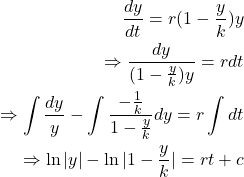
when ![]() then
then ![]() remains in this interval for all time. Thus we can remove the absolute bars and write that
remains in this interval for all time. Thus we can remove the absolute bars and write that
(k) 
Using initial conditions ![]() when
when ![]() we have
we have
![]()
Putting this value of ![]() in equation (k) we get
in equation (k) we get
(S) ![]()
After doing some calculations, we get from equation (S)
(D) ![]()
Which is the solution of Verhulst logistic model. In this model we see that when ![]() ,
, ![]() and when
and when ![]() ,
, ![]() .
.